These top 40 Excel Interview Questions will help you to win your Interview and get a Job. We wrote all types of questions from all the fields of Excel. We tried to cover formulas and functions as well. To prepare for an Excel interview you can go through these questions. It will definitely help to give you more exposure to which types of questions will be asked in your interview if you are a beginner.
Basic Excel Interview Questions
Microsoft Excel as we all know is a spreadsheet or a computer application that allows the storage of data in the form of a table. Excel was developed by Microsoft and can be used on various operating systems such as Windows, Mac OS, IOS and Android, etc.
Some of the important features of excel are the availability of graphing tools and built-in functions. It allows data analysis through tables, charts, filters, etc. It also allows data validation.
The area that falls under the intersection of row and column is known as a cell. The total number of rows that are available in Excel is 10,48,000,576 and the total number of columns is 16,000,384. So the total number of cells will be the multiplication of a number of rows and columns.
A spreadsheet is a collection of cells that help you manage the data. A single workbook may have more than 1 spreadsheet.
The cell address is refer to the address that is obtained by the combination of row number and column letter. So each excel may have a unique address.
Yes, to add the new cell you have to click on the cell where you want to insert a new cell. Now right-click on that cell and click on insert cell.
Yes, In order to format the cells you can use the command under font group under the HOME tab.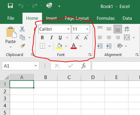
Yes, To add a comment on a cell only you have to right-click on the cell and choose the new comment option.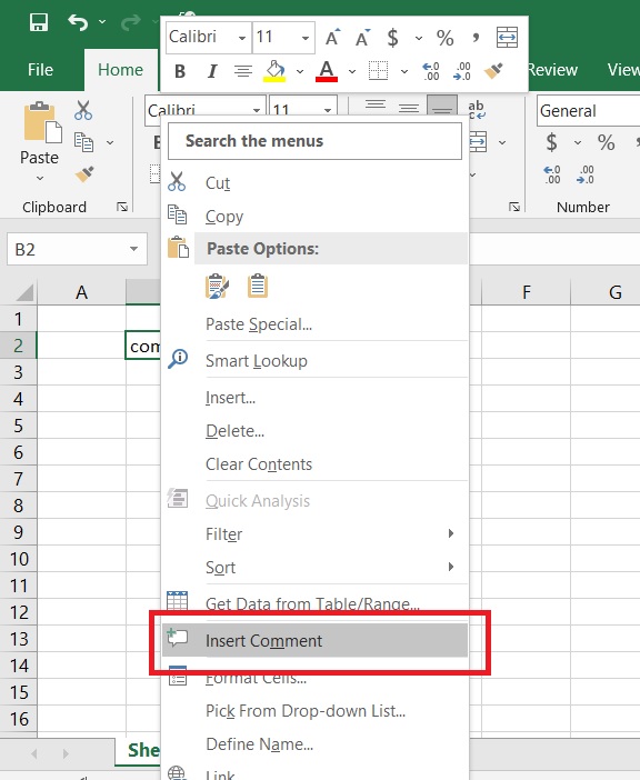
Yes, You can insert new rows and columns by just selecting a row or column and right-click and select the insert option.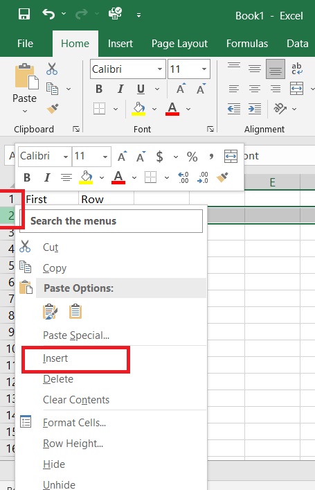
The ribbon is basically a key interface with excel and it appears at the top of the window. It consists of Home, Insert, Page layout, etc.
Go to the view tab and select the freeze pane option.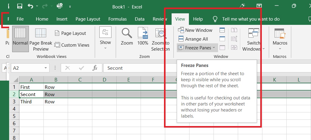
Yes, the Workbook can be protected. You can protect the sheet from being edited, deleted, hidden, or unhidden.
To do that all you have to do is right-click on any of the sheets present in the workbook and then click on the select all sheet option. After this, if I apply any format to any sheet it will automatically apply to other sheets.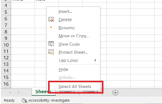
Whenever you copy formulas in excel the address of the reference cells gets modified automatically in order to match the position where the formula has been copied. Now, this is done by a system called relative cell addresses.
To do this you must make use of mixed cell references.
Yes, you can protect the required cell and the whole sheet. To do this select the cell you want to protect and go to font group and select protection and select hidden and now go to review and select protect sheet option.
Select the area in which you intend to give a name Go To the formula tab and select the define name command and give a name.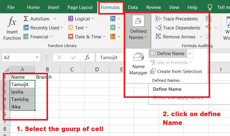
Excel allows you to automate the task that you do regularly by recording them into Macro. Macro is an action that you can perform n a number of times.
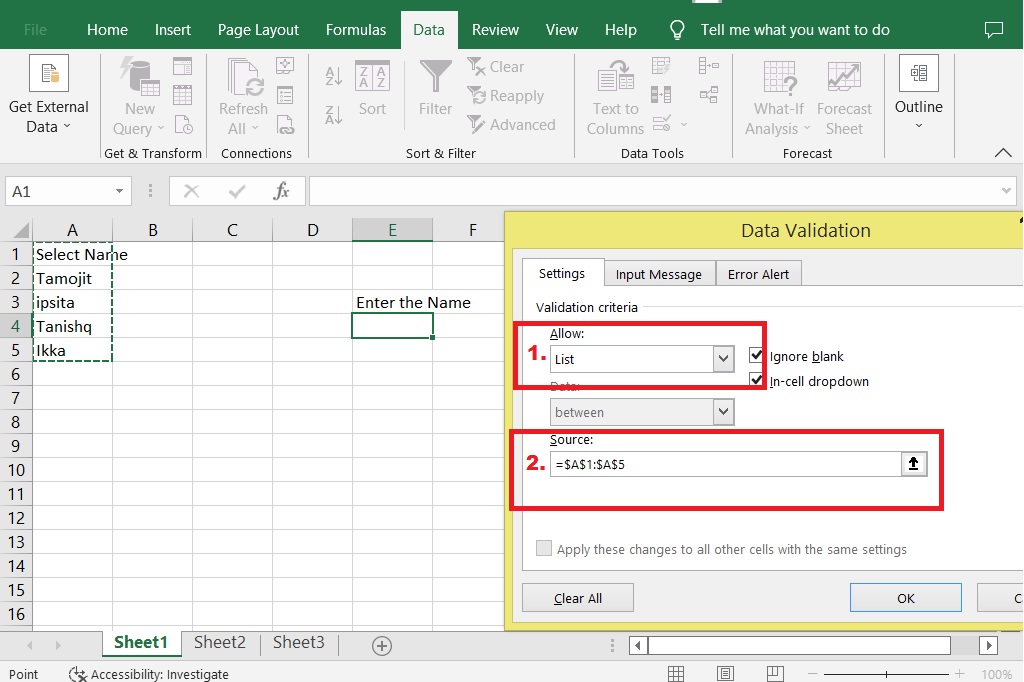
To create Drop Down go to the Data tab and select the data validation command. Select the list and provide the source, and press ok.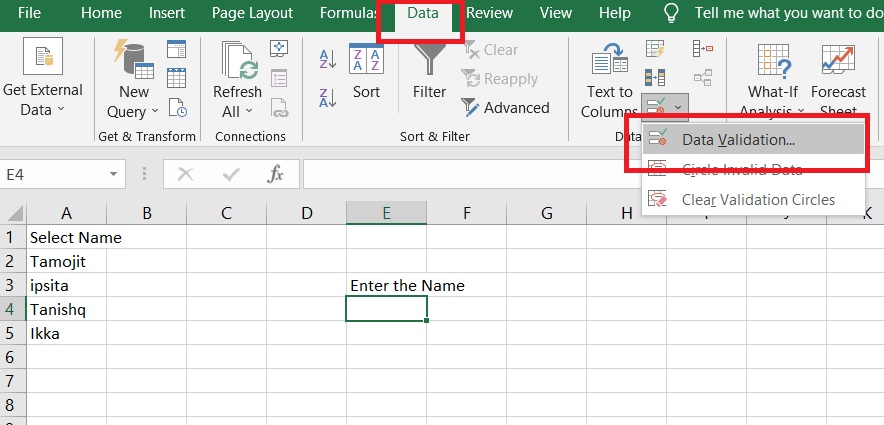
Pivot Tables and Pivot Charts Interview Question in Ms-Excel
Pivot tables are statistical tables that condense those tables that have extensive information. The summary can be based on any field. The pivot table represents that in an intelligent and simple manner.
Some of the important features of Pivot Tables are they allow the display of exact data that you have to analyze. They provide various angles in order to view the data. They allow you to focus on important details. Comparison of data is very handy and pivot tables can detect different patterns, relationships, etc.
They can also create instant data accurate reports and serve as the base for pivot charts.
First, you have to prepare data in tabular format. First, you have to arrange data in rows and columns the first row should contain a unique heading for each of the columns and the column should have one type of data present in them. The rows must have a data for single recording and there should be no blank rows. Columns should not be completely empty and the data for creating a pivot table should be separated from the other data present on that sheet.
MS Excel charts are data visualization tools. That helps you visualize the data in various ways. These charts can be of any type such as Bar, Pie, Area, Line, Donut, etc.
Yes, you can create pivot tables using one or more based tables, but you have to put the tables in the same worksheet.
Yes, If both the sheets are from the same workbook you can create the pivot table from the tables present in different sheets.
Yes, It is possible to see the details of the result shown in the pivot tables. All you have to do is double-click on any of them. And you will see that excel creates a new sheet about that result.
Excel pivot tables allow you to filter data according to your requirements. To this, only you to do is place the field on which base you want to filter the data. Then filter the data according to your choice.
Open up the drop-down list present for the row labels or the column labels then click on more sort options, then go to more options and uncheck the box that says sort automatically every time a report is updated, and click OK.
Formulas And Functions Interview Questions in MS-Excel
Functions are used to perform specific tasks. Excel has many built-in functions that are used to calculate the results of various formulas, thereby helping in time conservation. Also, these functions make it very easy to execute formulas, which have been if you go to manually write down.
Functions are categorized on the basis of Finance, Logic, Text, Date & Time, Math and Trigonometry, Lookup and reference, Database, Engineering, Cube, and Web Base Functions.
Formulas in Excel followed by BODMAS rule, which is Brackets, Order, Division, Multiplication, Addition, and Subtraction.
The sum function takes the ‘N’ number as a parameter and it Returns the sum by adding each of them.
SumIf Function Takes the ‘N’ number as a parameter and it returns the sum by adding those values that match the criteria.
In Excel, there are five types of count functions that are COUNT, COUNTA, COUNTBLANK, COUNTIF, and COUNTIFS.
a. Count Function returns the total number of numerical cell that is present in the range.
b. CountA function returns the total number of value cells present in the range.
c. CountIf function counts the number of cells present in a range that matches the criteria.
d. CountBlank function counts the total number of blank cells present in the range.
The countIfs function allows counting the number of cells by specifying a set of conditions in order to count them.
As we know, percentages are the ratio that is calculated as a fraction of a hundred.
In Excel to calculate the percentage, type equal to then obtained number divided by total number then hit enter. Now go to the Home tab and select the percentage command under the number group for that cell.
To calculate compound interest in excel, you can make use of the FV function. The FV function returns a future value of an investment based on periodic constant investment rates and payments.
In order to calculate the average, you have to use the average function and specify the range in the function.
Vlookup is a function present in Excel used to look up and bring forth data from a given range. V stands for Vertical and to use this function data should be arranged vertically. Vlookup is very useful when you have to find some piece of data from a huge amount of data.
Vlookup Function takes the Lookup value and searches for it in the leftmost column. When the first occurrence is found. It moves right. Returns a value from the given column. Can return exact and approximate matches.
For an exact match, you have to set the range lookup value to false.
To calculate an approximate match in VLOOKUP you have to set the range lookup value to true. And then it starts searching for the value in the left-most column and it stops at the next large value and moves to the right.
Yes, you can use Vlookup for multiple tables as well. In case you have to look up values, create name ranges for each of the tables and then use the IF function to select between each table based on some of the given conditions.
To perform the horizontal lookup you have to use the HLOOKUP function. Hlookup function just like the vlookup function takes a lookup value from the table array and instead of a column index number, it takes the row index number as the parameter value.

